Pop Gen Analysis

dDocent was used for QC, assembly, mapping and SNP calls on raw ddRAD data. dDocent SNP filtering pipeline plus rad haplotyper was used for filtering SNPs. Input file: SNP.DP3g95p5maf001.HWE.filtered.vcf.gz

Outlier detection

pcadapt provides statistical tools for outlier detection based on Principal Component Analysis (PCA)

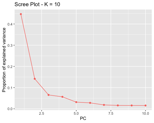
1. Choosing the number of principal components:

The ideal pattern in a scree plot is a steep curve followed by a bend and a straight line. Eigenvalues corresponding to population structure lie on the steep curve. By Cattell’s rule it is recommended to keep PCs that correspond to eigenvalues to the left of the straight line. K=2 was the choice made.

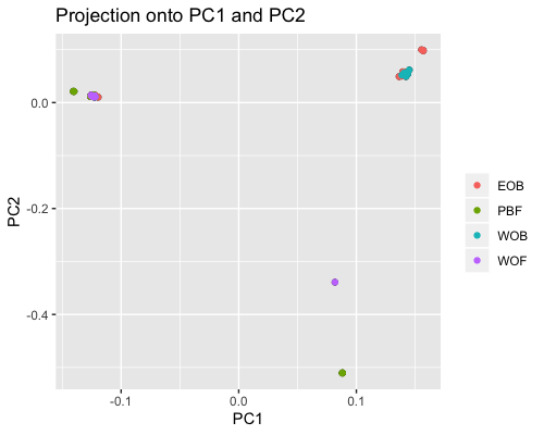
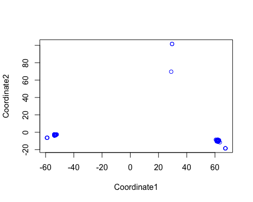
2. PCA based on scores:

Looking at scores the outliers are: WOF217, PBF165, PBF167, PBF168. Generally PC1 splits samples by back and fringe reef but some EOB/WOB samples wind up in fringe and one PBF160 sample in the back reef group.

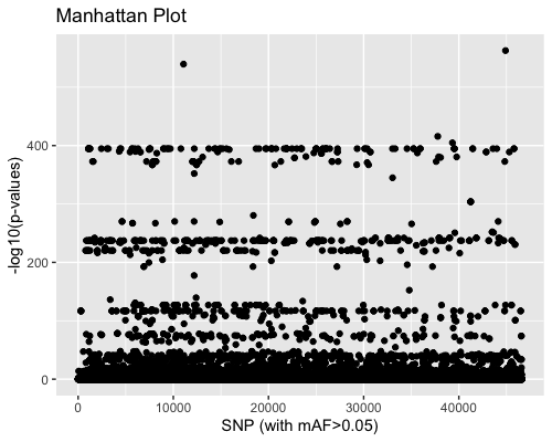
3. SNP distribution:

Mahattan plot shows the high number of outliers.

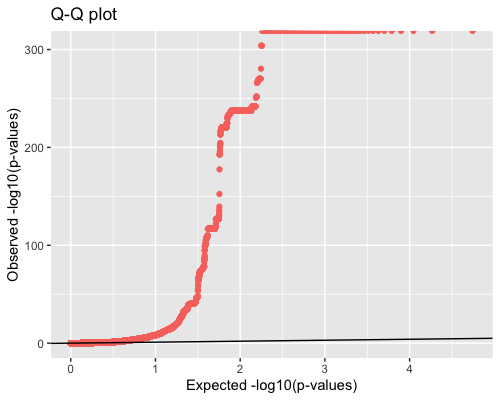
4. Distribution of pvalues:

Q-Q plot shows relation between observed and expected pvalues.

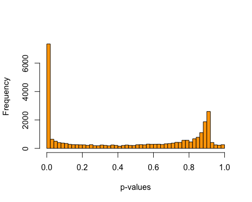
5. Histogram of pvalues:

Excess small pvalues indicates presence of outliers.

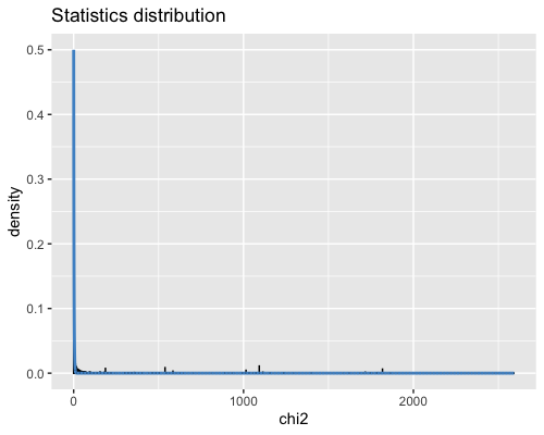
6. Histogram of the Mahalanobis distance:

This is a test statistic for detecting outlier SNPs that uses a multi-dimensional approach that measures how distant is a point from the mean.

MDS

DAPC

find.clusters identifies 5 clusters of sizes 4,4,4,20,26:

1. EOB_176,EOB_492,EOB_493,EOB_494
2. PBF_157,PBF_489, PBF_490, PBF_491
3. PBF_165, PBF_167, PBF_168,WOF_217
4. EOB_177,EOB_178,EOB_182,EOB_183,EOB_184,EOB_186,EOB_188,EOB_191,PBF_160,WOB_41,WOB_42,WOB_45,WOB_47,WOB_48,WOB_49,WOB_50,WOB_59,WOB_60,WOB_62,WOB_65
5. EOB_174,EOB_175,EOB_185,EOB_189,EOB_190,EOB_192,PBF_158,PBF_161,PBF_164,PBF_169,PBF_171,PBF_172,WOB_35,WOF_224,WOF_225, WOF_232, WOF_234, WOF_236,WOF_237,WOF_238,WOF_239,WOF_240,WOF_241,WOF_243,WOF_244,WOF_245.

Fst

1. fst for all individuals together:

fstat function from hierfstat R package was used to calculate Fst of all the data

           pop       Ind
     Total 0.1675746 0.3774758
     pop   0.0000000 0.2521562

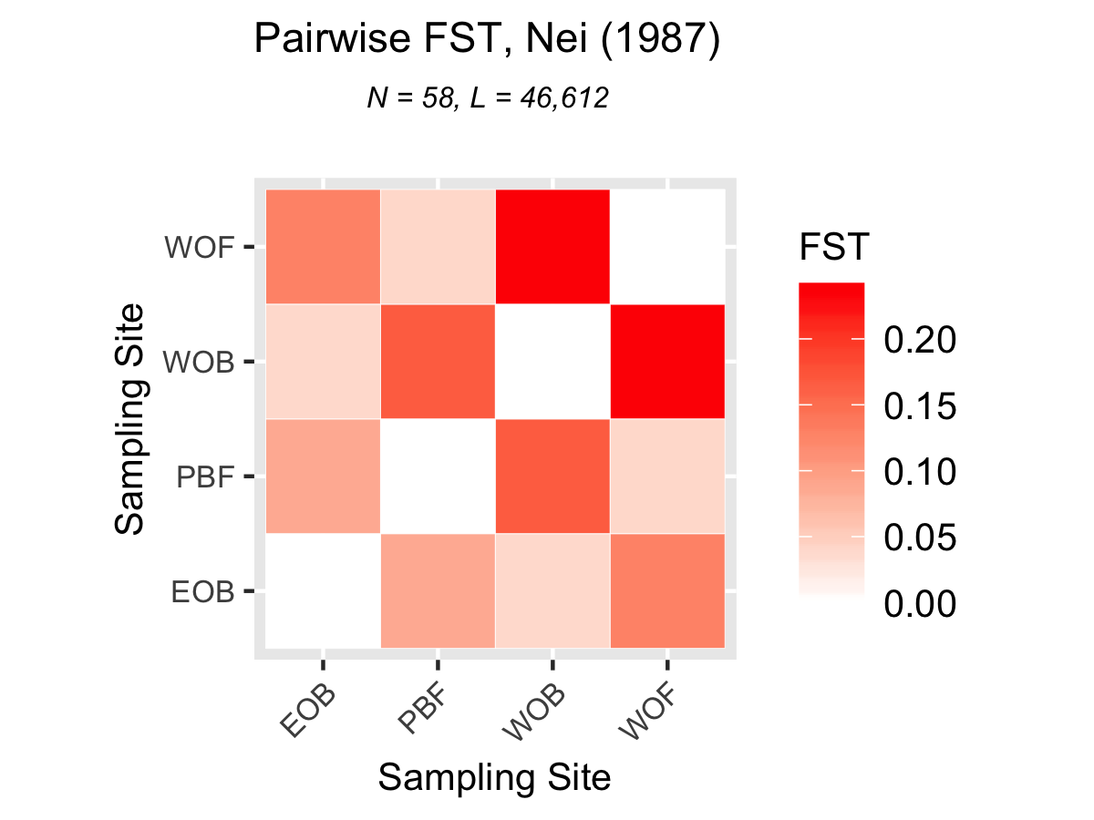
2. Pairwise Fst by location:

This was calculated using the Nie method. All four locations were compared to each other.

3. Pairwise FST by reef type:

This also calculated by the Nie method. Back vs Fringe comparison FST: 0.1261697.